Excel Tips and Tricks / Business Reporting Question: I would like to have two fields for analyzing sales in the PivotTable, one in a percentage format and the other in a value format. How can I accomplish this?

Answer: By using the Value Field Settings

Why: To display the Product sales field in percentage and value formats

Applies To MS Excel 2003, 2007, 2010

1. For an example on how to create pivot tables refer to the link given below;

Creating a Pivot Table.

2. Select any cell in the PivotTable as given in the above example.

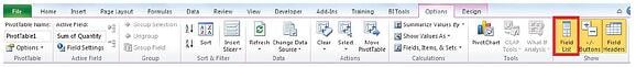
3. If the Pivot Table field list is not displayed select field list button on the Options tab in Excel.

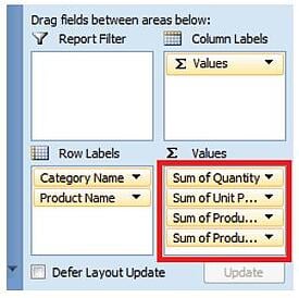
4. Add the product Sales column to the values area again. Refer to the screen shot given below.

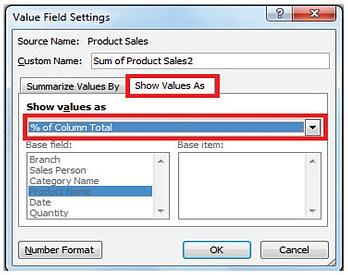
5. Change the Sum of Product Sales2 field to a %;

(a) Right click on the field Sum of Product Sales 2 in the pivot table.

(b) Select values field setting and select as below.

Ms Excel 2007/ Ms Excel 2010

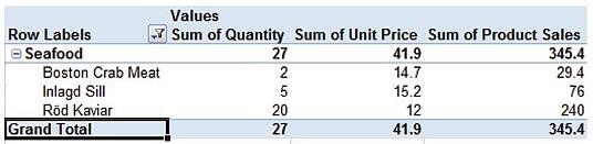
5. The result will be the pivot table shown below.

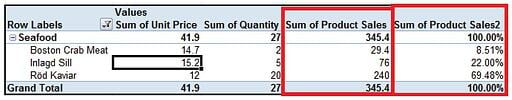
The analysis of sales by percentage and values can thus be performed.One can easily compare the sales of the various products by looking at the percentage column for the product sales.

You can now change the name of the Fields to be more appropriate. I.e. Sum of Product Sales = Product Sales Total; Sum of Product Sales2 = % of Total Sales.